Accuracy is the number everyone quotes and the one that tells you the least. Two models can post the same headline figure and still be nothing alike to deploy. One is twice as unfair. Another folds under distribution shift, or needs 13 GB of GPU memory to score a few hundred rows. So we ran a wider study on TabFM, Google's latest tabular foundation model, which now ships in TabTune with zero-shot, meta-learning, supervised fine-tuning, and PEFT adaptation behind one API. 

We lined it up against two strong in-context learners, TabPFNv3 and TabICLv2, and a gradient-boosted tree baseline, across ten datasets spanning oncology, finance, chemistry, speech, neuroscience, astrophysics, energy, and census data.

Here is the full story: where TabFM wins, where it ties, and where it costs you something the accuracy column never shows.

The setup: ten datasets, four TabFM arms

Everything in this study ran on a single NVIDIA A100 (80 GB), The suite is ten binary-classification datasets from OpenML and scikit-learn, chosen to spread across domains and sizes rather than to flatter any one model: from 569 rows of tumour measurements to 48,842 rows of census records, and from 5 features to 41.

‍The model grid: TabFM in four adaptation regimes - zero-shot, episodic meta-learning, supervised fine-tuning, and PEFT (LoRA, r=8, α=16, dropout 0.05) -  all driven through TabTune's TabularPipeline with one API. Fine-tuning is deliberately conservative: 3 epochs at a learning rate of 2e-6, episodic support/query sampling on the real differentiable in-context forward. Comparators are TabPFNv3 and TabICLv2, both zero-shot, plus a GBDT baseline (scikit-learn HistGradientBoosting, default settings).

The protocol: stratified 75/25 train/test splits with an absolute cap on test size (so the big datasets keep a large training pool for the scaling sweeps), fixed seed 42 throughout, datasets subsampled to keep single-run turnaround practical. Zero-shot inference uses the vendored engine's full preprocessing and 32-member permutation ensemble. 

1 · On accuracy, the tie is gone. The foundation models win

Ranking the four systems across all ten datasets, TabFM takes first place with a mean rank of 1.65, ahead of TabPFNv3 (2.15), TabICLv2 (2.60), and the GBDT (3.60). The separation is real this time: TabFM sits more than a Nemenyi critical difference (1.48 at α=0.05) clear of the tree.

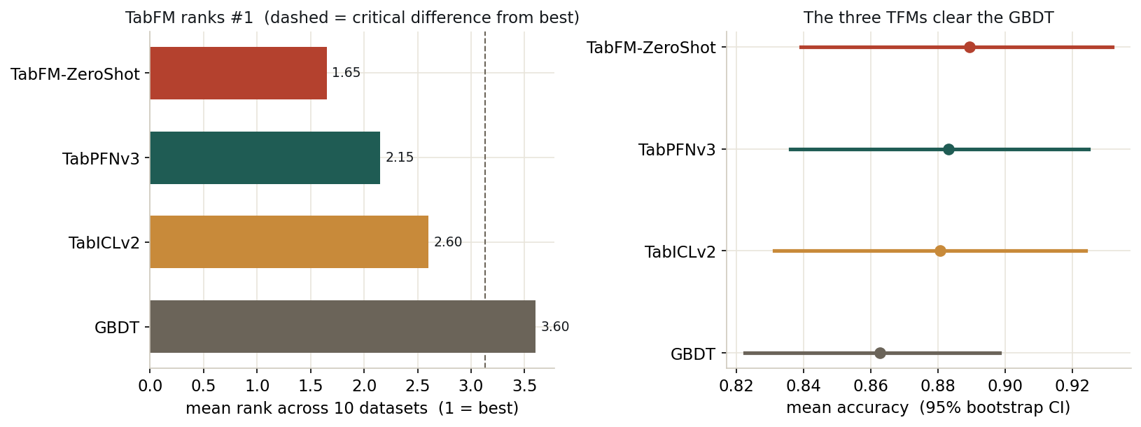
Figure 1 : Left: mean rank across 10 datasets (lower is better); the dashed line marks a critical difference from the top model. Right: bootstrap 95% confidence intervals on mean accuracy.

The credibility check mostly confirms it. A paired bootstrap over datasets puts the GBDT − TabFM gap at −2.68 points with a 95% CI of [−4.5, −1.1] that never crosses zero: the tree loses in 100% of resamples. TabPFNv3 and TabICLv2 also clear the tree. Among the three foundation models the picture is tighter. TabFM edges TabPFNv3 by 0.6 points, and that CI straddles zero. Its 0.9-point edge over TabICLv2 excludes zero by a hair in the bootstrap, but doesn't survive the Holm-corrected Wilcoxon test. The foundation models beat the tree; between the three of them, TabFM leads on rank but the accuracy differences are at the edge of what ten datasets can resolve.

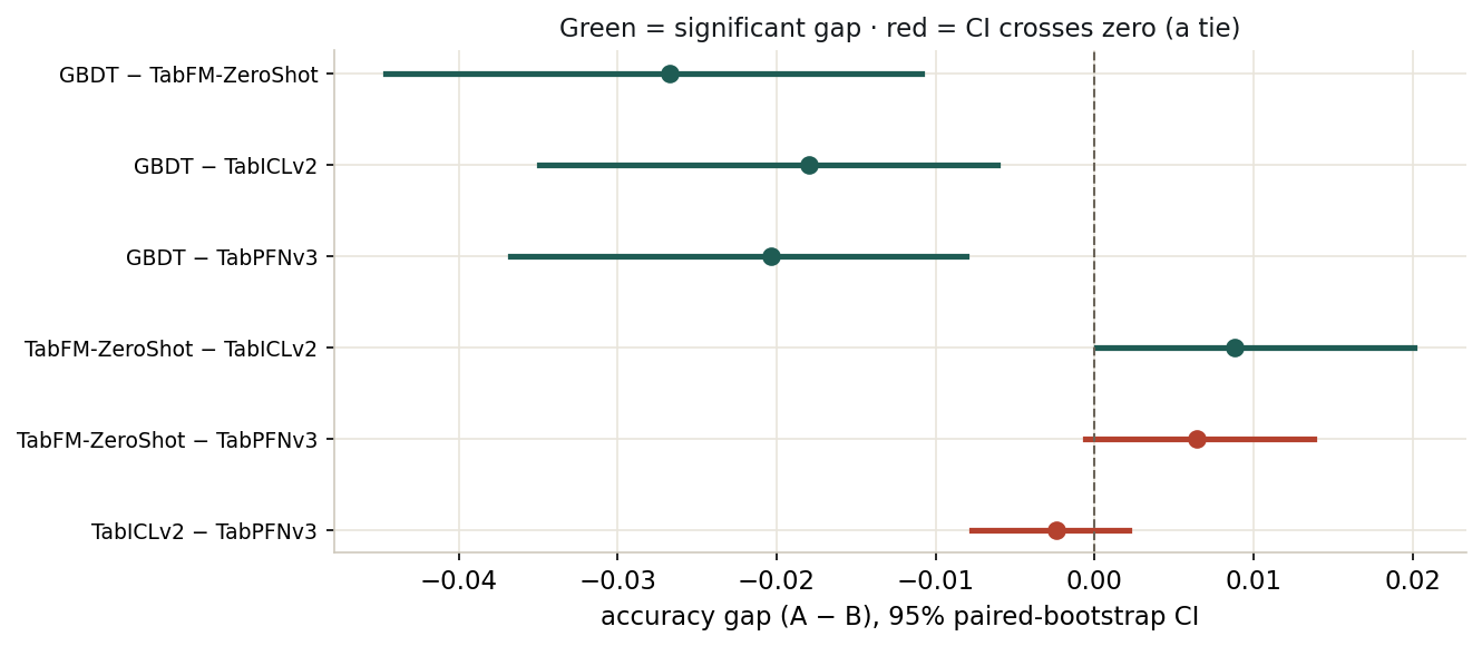
Figure 2 : Pairwise accuracy gaps with paired-bootstrap 95% CIs. Green intervals exclude zero (a real difference); red ones straddle it (a tie). Every foundation-model-vs-GBDT gap is green.

2 · The low-data regime is where TabFM earns its keep, but it's dataset-dependent

Where does that edge come from? Mostly the low-data regime. At 20 training rows TabFM shows up already knowing what tabular data tends to look like, while the tree is still hunting for structure. On breast_cancer the gap is enormous: +28 points at 20 rows. On electricity it's +15, on qsar-biodeg +12.5, on eeg-eye-state and diabetes about +6.

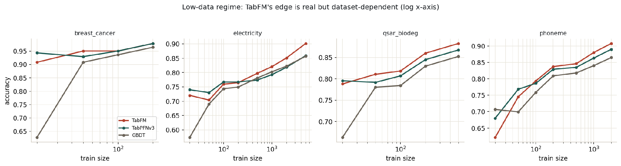
Figure 3 — Accuracy vs training-set size (log x-axis) on four representative datasets. TabFM's advantage is largest at the smallest sizes and narrows as data grows.

But breadth tells a fuller story than any single dataset.. Across all ten datasets the 20-row advantage is mixed: big wins on some, and small losses on others. Phoneme is −8.5 points, credit_g −0.8, bank_marketing −0.1. The prior helps most when the problem resembles what the model was pre-trained on, and can hurt when it doesn't. This is the nuance a single-dataset demo always hides.

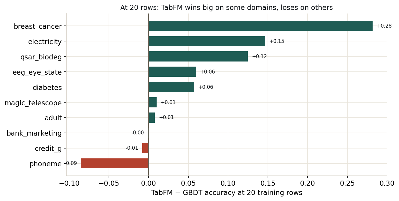
Figure 4 : TabFM minus GBDT accuracy at 20 training rows, all ten datasets. Teal = TabFM wins, red = the tree wins. The advantage is real but far from universal.

3 · Fine-tuning and PEFT cost you fairness

Adaptation is why you ship TabFM as a library and not a bare checkpoint, and it is where the finding that matters most for deployment shows up. On the adult census task, zero-shot TabFM is 87.1% accurate with an equalized-odds gap of 0.111. Fine-tune it and accuracy ticks up to 87.2% while the odds gap widens to 0.118. On credit_g the pattern is sharper: SFT and PEFT add 0.4 points of accuracy while pushing the equalized-odds gap from 0.071 to 0.115, a 62% increase in unfairness for an accuracy gain nobody would notice.

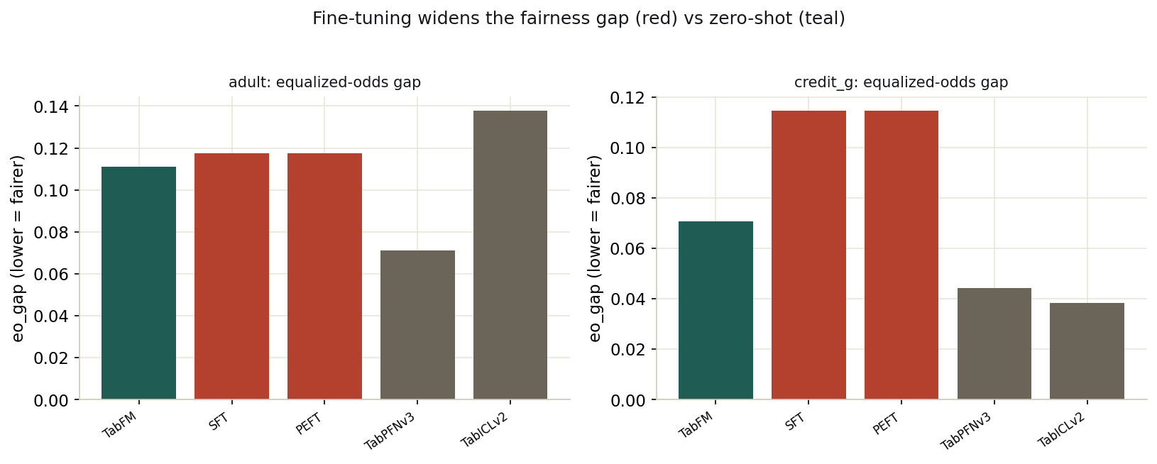
Figure 5 :  Equalized-odds gap by model on the two datasets carrying a protected attribute. Red bars (SFT / PEFT) sit higher than the teal zero-shot baseline. Lower is fairer.

‍

‍

At the conservative learning rate we used (2e-6), the adaptation arms move only a handful of test predictions ,  meta-learning moved none, which is why its row is identical to zero-shot, and SFT and PEFT landed on the same flips. Treat the erosion as directional evidence at this scale, not a precise effect size.

Three caveats keep this honest. Meta-learning left the gaps untouched, so not every adaptation method does this. The absolute deltas come from a small number of flipped predictions, because we deliberately fine-tune gently; a more aggressive recipe could look better or much worse. And on credit_g, TabPFNv3 and TabICLv2 zero-shot were fairer than TabFM (odds gaps of 0.044 and 0.038). The lesson isn't that foundation models are unfair. It's that adaptation optimises whatever loss you give it, and fairness usually isn't in that loss. Check the gap before you fine-tune and again after. TabTune now gives you both the fine-tuning and the audit.

4 · The signature test: does the answer change if you shuffle the columns?

Here's a question no leaderboard asks. These models claim to be invariant to the order of their features and their in-context rows, but the architecture only approximates that by ensembling over permutations. So we shuffled the columns, shuffled the support rows, and measured how often the prediction flips.

The reassuring news: instability is low everywhere. Under column permutation TabFM changes its answer on just 0.26% of rows, roughly 4× steadier than TabPFNv3 and TabICLv2 (

‍

both around 1%). Row order is a different story: there TabICLv2 is the calmest (0.07%), with TabFM at 0.36%. So no model wins every axis. TabFM owns column shuffles, TabICLv2 owns row shuffles, and all of the rates are small. Still worth knowing they're non-zero before you promise a customer a deterministic answer.

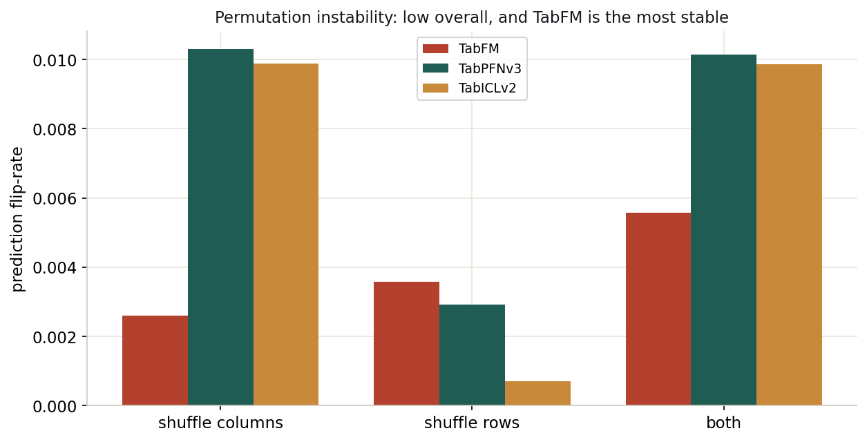
Figure 6 : Prediction flip-rate under permutation of columns, rows, or both. Lower is more stable. TabFM is steadiest under column shuffles; TabICLv2 under row shuffles.

‍

5 · The context lottery

An in-context model has no weights to train; its whole 'fit' is the support set. Which rows you happen to show is itself a hyperparameter. With a 50-row context, two random draws on breast_cancer swing accuracy across a 9-point range (88.1% to 97.2%). On eeg-eye-state the 50-row spread is even wider, almost 17 points. The good news: the lottery is tameable. Push the context to 200 rows and breast_cancer's spread collapses to about 2 points; at 500 rows most datasets sit under 2.

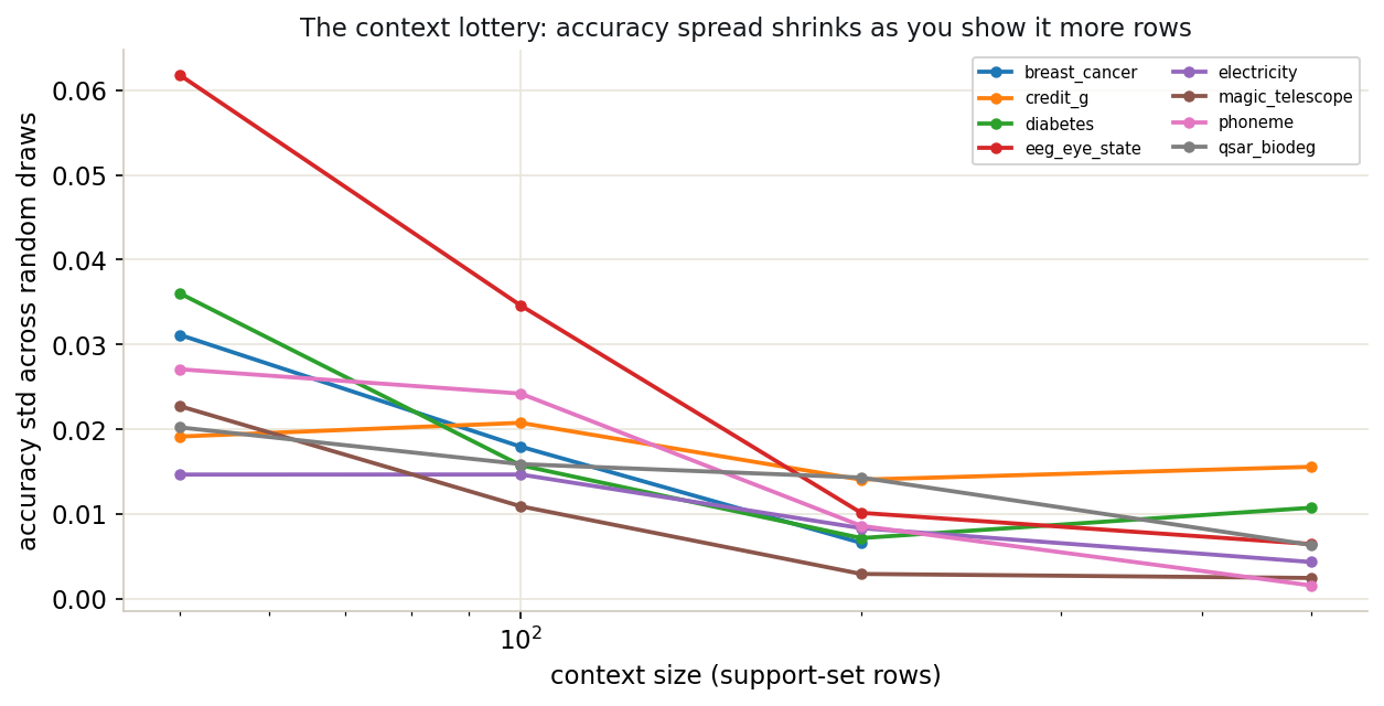
Figure 7 :  Accuracy standard deviation across random support-set draws (TabFM), by context size. More context rows means a smaller lottery. Log x-axis.

‍

6 · Robustness depends entirely on how you break things

We stressed the models along four axes. Three barely dent performance: label noise, feature noise, and missing values all leave robustness scores of 0.89 or higher, with the three models within a whisker of each other. Then there's a covariate shift, and it's a cliff. Every model collapses to about 0.68. Shift the input distribution far enough and the in-context prior that makes these models strong in the low-data regime becomes a liability. If your production distribution drifts, none of the three saves you. That's a monitoring problem, not a model choice.

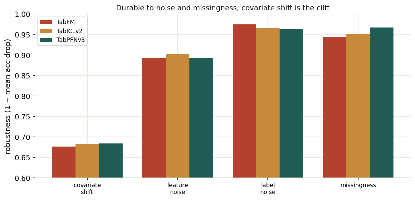
Figure 8 : Robustness score (1 − mean accuracy drop) by corruption axis. Durable to noise and missingness; covariate shift is the shared failure mode.

‍

7 · Serving is expensive, so distillation is the deployment path

TabFM is costly to serve: 14–21 rows per second and roughly 13 GB of peak GPU memory regardless of dataset size, versus thousands of rows per second on CPU for a tree. The fix is distillation, and mostly it works. On breast_cancer a distilled MLP keeps 97.9% of the teacher's accuracy while running about 2,000× faster; the LGBM student keeps 97.1% at 830×. Phoneme distils to 93.5% (LGBM) and 91.1% (MLP, at a wild 18,700× speed-up). Electricity is the cautionary tale: the LGBM student holds 90.5%, but the MLP drops to 84.2%. Retention is dataset- and student-dependent, so validate per dataset before you ship the student.

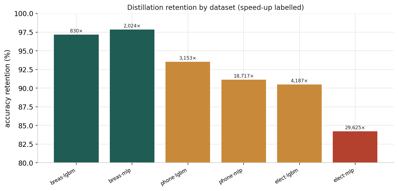
Figure 9 : Distillation accuracy retention by dataset and student type, with speed-up factor labelled above each bar. Teal ≥ 95%, gold ≥ 90%, red below.

‍

8 · Decision costs: the ranking that refused to invert

One more test, because accuracy silently assumes a false negative costs the same as a false alarm. We re-ranked the three foundation models by expected cost per row under three cost regimes: symmetric (1:1), moderate (5:1), and severe (10:1) false-negative penalties, each at its own cost-optimal threshold. We were hunting for a rank inversion, the kind of result that makes model choice depend on the application. We didn't get one. TabFM is the cheapest model under all three regimes (0.105, 0.226, and 0.279 cost per row on average), with TabPFNv3 second and TabICLv2 third, and the ordering never budges. It's a dull table, and a useful one: for these datasets the accuracy leader is also the cost leader.

‍

The verdict

Start with the scoreboard, because this time it's unambiguous. On a real 10-dataset benchmark, TabFM ranks first of four systems, and the foundation models beat the gradient-boosted tree by 1.8 to 2.7 accuracy points with confidence intervals that never touch zero. The tree loses in 100% of bootstrap resamples. The old 'foundation models merely tie GBDTs' folklore was an artifact of benchmarks too small to resolve the difference. It's resolved now.

The deeper result is that the accuracy column was the least interesting one we measured. The same model that tops the leaderboard gives up 28 points of low-data advantage on one dataset and concedes 8.5 on another. Its fine-tuned variants buy 0.4 points of accuracy at the price of a 62% wider equalized-odds gap. Its predictions wobble, slightly but measurably, when you shuffle its columns. Its accuracy at a 50-row context is a lottery with a 9-to-17-point spread. And every model we tested, TabFM included, falls off the same cliff under covariate shift. A leaderboard compresses all of that into one number and calls it a ranking. Every experiment in this study says that number is the start of due diligence, not the end.

So here is the deployment playbook this study leaves you with. Reach for TabFM when labels are scarce; that's where the pre-trained prior pays for itself, and where the tree simply cannot compete. Give it as much context as you can afford, because 200 rows buys the lottery down to noise. If you fine-tune, audit fairness before and after, and prefer meta-learning when the gaps matter. Serve it distilled: a student that keeps 97% of the teacher at 2,000× the speed is the difference between a demo and a product, but validate retention per dataset before you ship. And whatever your cost matrix looks like, the cheapest model here is also the most accurate one, under every regime we tried.

The bottom line: TabFM is the strongest tabular foundation model we've measured, and TabTune is what made measuring it possible,  one API for zero-shot, meta-learning, SFT, PEFT, and every audit in this study. TabFM wins the accuracy column. Everything else in this post is the part you still have to check per deployment.

‍